Lab 3 - with solutions

Please note that there is a file on Canvas called Getting started with R which may be of some use. This provides details of setting up R and Rstudio on your own computer as well as providing an overview of inputting and importing various data files into R. This should mainly serve as a reminder.

Recall that we can clear the environment using rm(list=ls()) It is advisable to do this before attempting new questions if confusion may arise with variable names etc.

Example 1

In this example we want to determine whether there is any difference between the driving reaction times after drinking water, coffee and alcohol in the Kruskal-Wallis (Reaction Times) dataset. Please follow the steps below:

Firstly, we input the dataset into R and check it using the ``head” command (recall this provides the first 6 entries). We use the gdata package to import the Excel file.

library(readxl)
Reaction<-read_excel(file.choose())

head(Reaction)

# A tibble: 6 × 2
  `Reaction Times` `Drink Groups`
             <dbl>          <dbl>
1             0.37              1
2             0.38              1
3             0.61              1
4             0.78              1
5             0.83              1
6             0.86              1

We next perform a test of normality on the standardized residuals to determine which method should be used. If the residuals are normally distributed and we have homogeneity of variances (Levene’s test) then we would use ANOVA. The following code creates and performs tests of normality on the residuals.

anova_model<-aov(Reaction$"Reaction Times"~Reaction$"Drink Groups")
summary(anova_model)

residuals<-rstandard(anova_model)
shapiro.test(residuals)


    Shapiro-Wilk normality test

data:  residuals
W = 0.89219, p-value = 0.005437

library(nortest)
lillie.test(residuals)


    Lilliefors (Kolmogorov-Smirnov) normality test

data:  residuals
D = 0.14947, p-value = 0.08544

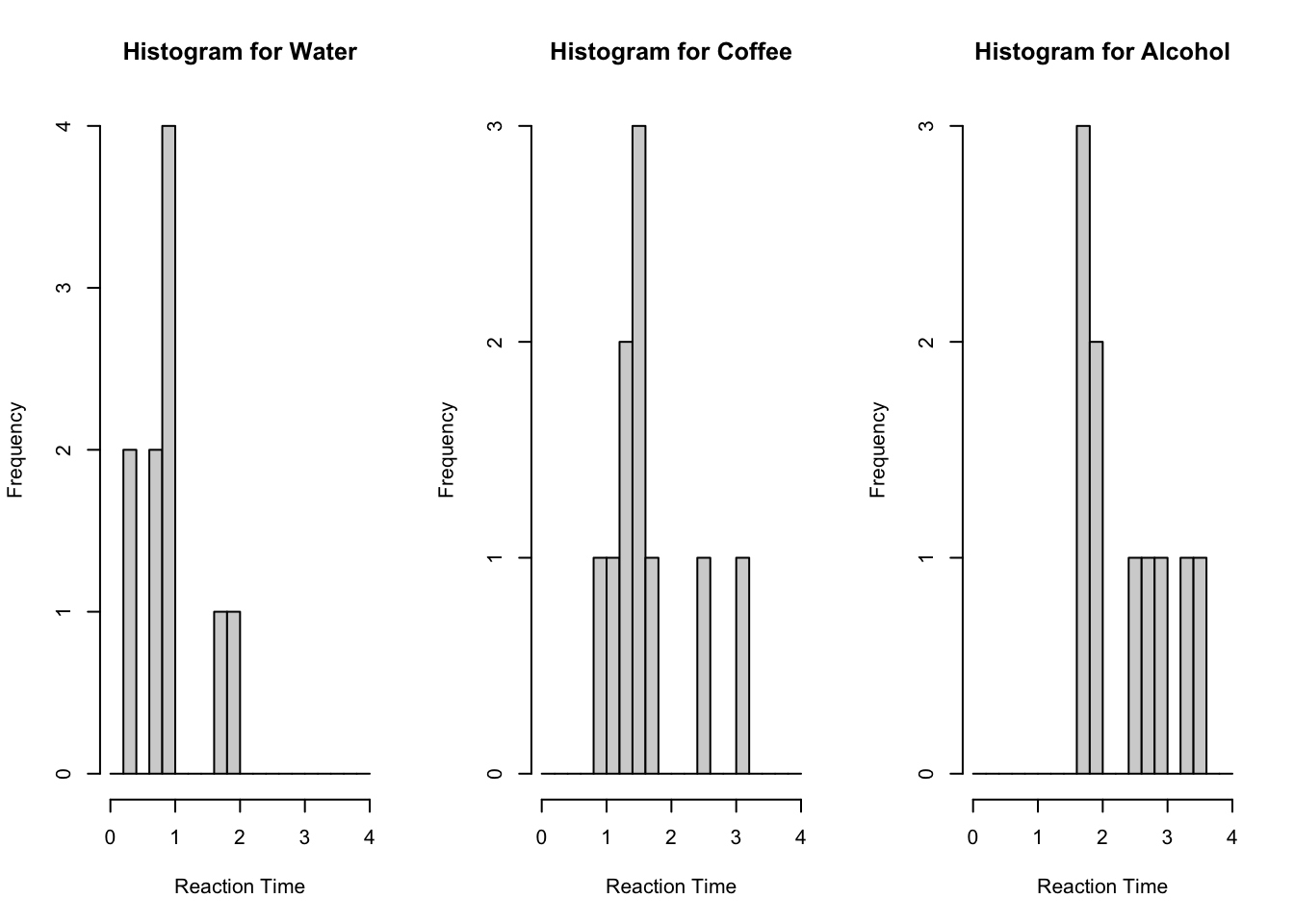
Clearly the residuals are not normally distributed, therefore we must use the nonparametric equivalent of the ANOVA procedure, i.e. the Kruskal-Wallis H-test. In order to determine the correct hypotheses, we next investigate the shapes of the distributions of the groups using histograms:

DrinkTypes<-factor(Reaction$"Drink Groups",c(1,2,3),labels=c('Water','Coffee', 'Alcohol'))
par(mfrow=c(1,3)) 
hist(Reaction$"Reaction Times"[DrinkTypes=='Water'], xlab='Reaction Time', 
     main='Histogram for Water', breaks=seq(from=0,to=4, by=0.2)) 
hist(Reaction$"Reaction Times"[DrinkTypes=='Coffee'], xlab='Reaction Time', 
     main='Histogram for Coffee', breaks=seq(from=0,to=4, by=0.2))
hist(Reaction$"Reaction Times"[DrinkTypes=='Alcohol'], xlab='Reaction Time', 
     main='Histogram for Alcohol', breaks=seq(from=0,to=4, by=0.2))

From the histograms we see that the groups seem to have similar shaped distributions, therefore use the following hypotheses:
- \(H_0:\) The medians of all groups are equal;
- \(H_1:\) At least one group has median not equal to the others.
Next we perform the Kruskal-Wallis H test.

kruskal.test(Reaction$"Reaction Times"~Reaction$"Drink Groups")


    Kruskal-Wallis rank sum test

data:  Reaction$"Reaction Times" by Reaction$"Drink Groups"
Kruskal-Wallis chi-squared = 16.322, df = 2, p-value = 0.0002856

As we have a significant result we undertake a Dunn post hoc test with Bonferroni correction.

install.packages("FSA")

library(FSA)

dunnTest(Reaction$"Reaction Times"~factor(Reaction$"Drink Groups"), method="bonferroni")

Dunn (1964) Kruskal-Wallis multiple comparison

  p-values adjusted with the Bonferroni method.

  Comparison         Z      P.unadj        P.adj
1      1 - 2 -2.095735 3.610569e-02 0.1083170553
2      1 - 3 -4.039053 5.366736e-05 0.0001610021
3      2 - 3 -1.943318 5.197773e-02 0.1559332006

You should see that there is a significant difference between drinks 1 and 3, i.e. between water and alcohol. We therefore report medians using the following code:

tapply(Reaction$"Reaction Times",Reaction$"Drink Groups",median)

    1     2     3 
0.845 1.445 2.250

Exercise 1

The Diets dataset contains data on the weight loss of 3 groups of participants who took park in 3 different diets. Determine whether there is any difference in the effectiveness of the diets, fully justifying the method used.

Solution

We first import the data.

Diets<-read.csv(file.choose(), header = T)

In order to determine whether we need to use a parametric or non-parametric technique, we investigate the normality of the residuals.

anova_model2<-aov(Diets$Weight.Loss~Diets$Diet)
summary(anova_model2)

            Df Sum Sq Mean Sq F value Pr(>F)
Diets$Diet   1   12.0   12.00   0.369  0.552
Residuals   16  520.9   32.56

residuals2<-rstandard(anova_model2)
shapiro.test(residuals2)


    Shapiro-Wilk normality test

data:  residuals2
W = 0.89376, p-value = 0.04479

library(nortest)
lillie.test(residuals2)


    Lilliefors (Kolmogorov-Smirnov) normality test

data:  residuals2
D = 0.27639, p-value = 0.00078

The results indicate that the residuals do not appear to be normally distributed, hence we use the Kruskal-Wallis test (as we have 3 independent groups).
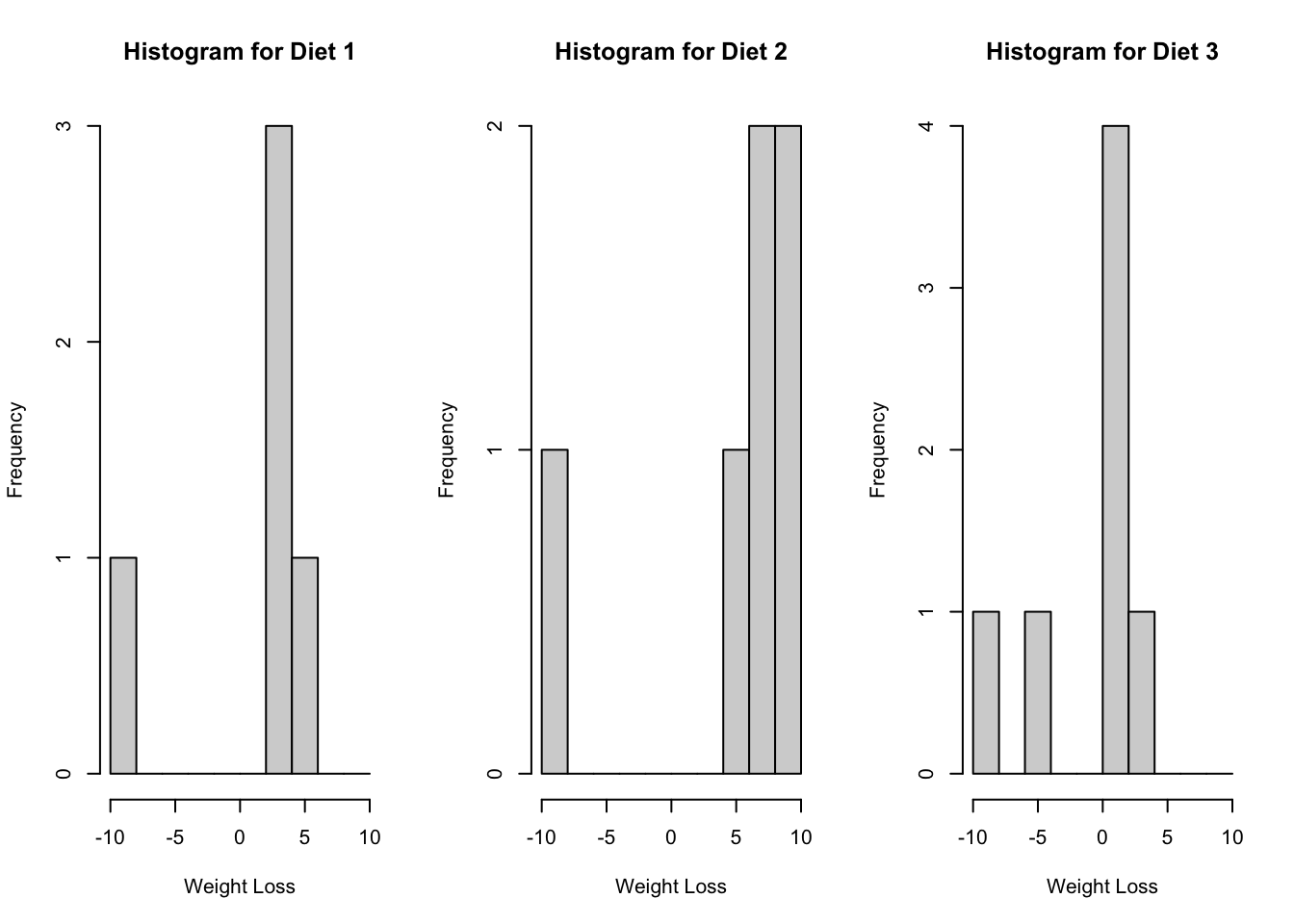
In order to identify the correct hypotheses, we need to investigate the shape of the distributions of the groups.

par(mfrow=c(1,3)) 
hist(Diets$Weight.Loss[Diets$Diet==1], xlab='Weight Loss', main='Histogram for Diet 1', breaks=seq(from=-10,to=10, by=2)) 
hist(Diets$Weight.Loss[Diets$Diet==2], xlab='Weight Loss', main='Histogram for Diet 2', breaks=seq(from=-10,to=10, by=2))
hist(Diets$Weight.Loss[Diets$Diet==3], xlab='Weight Loss', main='Histogram for Diet 3', breaks=seq(from=-10,to=10, by=2))

From the histograms we see that the groups seem to have similar shaped distributions, therefore we will compare medians in the Kruskal-Wallis test.

kruskal.test(Diets$Weight.Loss~Diets$Diet)


    Kruskal-Wallis rank sum test

data:  Diets$Weight.Loss by Diets$Diet
Kruskal-Wallis chi-squared = 6.5272, df = 2, p-value = 0.03825

As we have a significant result we undertake a Dunn post hoc test with Bonferroni correction.

install.packages("FSA")

library(FSA)
dunnTest(Diets$Weight.Loss~Diets$Diet, method="bonferroni")

Dunn (1964) Kruskal-Wallis multiple comparison

  p-values adjusted with the Bonferroni method.

  Comparison         Z    P.unadj      P.adj
1      1 - 2 -1.306966 0.19122413 0.57367240
2      1 - 3  1.075422 0.28218581 0.84655744
3      2 - 3  2.554352 0.01063857 0.03191572

This shows a significant difference between diest 1 and 2. We therefore report the medians of these groups.

tapply(Diets$Weight.Loss,Diets$Diet,median)

  1   2   3 
3.0 7.5 2.0

Example 2

In this example we will continue the example of determining whether a bonus scheme improves lateness in employees. Recall the data below:

Employee	Baseline	Month 1	Month
1	16	17	11
2	10	5	2
3	7	8	0
4	13	9	5
5	17	2	2
6	10	10	9
7	11	6	5

We will now use a Friedman test to determine whether there is any difference in the medians of these groups. Please follow the steps below in R:

We first input the data:

Baseline<-c(16,10,7,13,17,10,11)
Month1<-c(17,5,8,9,2,10,6)
Month2<-c(11,2,0,5,2,9,5)
LatenessData<-data.frame(Baseline,Month1,Month2)
LatenessData

  Baseline Month1 Month2
1       16     17     11
2       10      5      2
3        7      8      0
4       13      9      5
5       17      2      2
6       10     10      9
7       11      6      5

Next we check the normality of the residuals using the following code. We first need to upload the dataset Work Lateness.csv, which in a different format. (It is not as straightforward as in the Kruskal-Wallis case.)

LatenessNew<-read.csv(file.choose(), header=T)
LatenessNew
attach(LatenessNew)

anova_model3 <- aov(Lateness~Bonus+Error(EmployeeA))                                      
anova.model3.pr <- proj(anova_model3)
residuals<-anova.model3.pr[[3]][, "Residuals"]
shapiro.test(residuals)


    Shapiro-Wilk normality test

data:  residuals
W = 0.94283, p-value = 0.2478

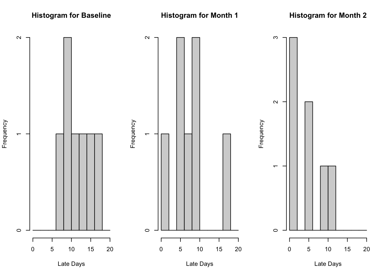
The residuals seem to be normally distributed, however we continue with the Friedman test as the sample size is small (and we will see shortly that the data are skewed). We next investigate the shapes of the group to determine the correct hypotheses.

par(mfrow=c(1,3)) 
hist(Baseline, xlab='Late Days', main='Histogram for Baseline', breaks=seq(from=0,to=20, by=2)) 
hist(Month1, xlab='Late Days', main='Histogram for Month 1', breaks=seq(from=0,to=20, by=2))
hist(Month2, xlab='Late Days', main='Histogram for Month 2', breaks=seq(from=0,to=20, by=2))

We see that the groups seem to have the same shaped distribution, hence we compare medians in the hypotheses. The histograms are all skewed, providing further evidence that non parametric techniques are not suitable. We now proceed with Friedman’s test. Note that we have to make a matrix out of the data to perform the test.

LatenessMatrix<-matrix(c(Baseline, Month1, Month2),ncol=3, nrow=7,dimnames = list(1 : 7, c("Baseline", "Month1", "Month2")))
LatenessMatrix

  Baseline Month1 Month2
1       16     17     11
2       10      5      2
3        7      8      0
4       13      9      5
5       17      2      2
6       10     10      9
7       11      6      5

friedman.test(LatenessMatrix)


    Friedman rank sum test

data:  LatenessMatrix
Friedman chi-squared = 10.231, df = 2, p-value = 0.006004

Since we have a significant result we perform a post hoc test. We use the Nemenyi post-hoc tests in the PMCMRplus package.

install.packages("PMCMRplus")

library(PMCMRplus)
kwAllPairsNemenyiTest(LatenessNew$Lateness~LatenessNew$Bonus)


    Pairwise comparisons using Tukey-Kramer-Nemenyi all-pairs test with Tukey-Dist approximation

data: LatenessNew$Lateness by LatenessNew$Bonus

  0      1     
1 0.0794 -     
2 0.0072 0.6646


P value adjustment method: single-step

alternative hypothesis: two.sided

You should come to the conclusion from this output that there is a significant difference between Baseline and Month2. We next report their medians using the code:

median(Baseline)

[1] 11

median(Month2)

[1] 5

Exercise 2

Determine whether there are any differences between the groups Overall score (Video A), Overall score (Video B), Overall score (Video C) and Overall score (Demo D) in the Public Awareness SPSS dataset.

Hint: Before performing the Friedman test you will need to create a matrix of the relevant variables. The following code may help you to do this:

AwarenessMatrix<-matrix(c(Awareness$TotalAGen, Awareness$TotalBdoc, Awareness$TotalCOld,
        Awareness$TotalDDEMO), nrow=20,ncol=4, dimnames = list(1 : 20, c("A", "B", "C", "D")))

You will then need to create another dataset with one column containing all the awareness scores and a corresponding label column. I would suggest exporting your matrix created above using the write.csv() command and making these changes in Excel, then re-import your new dataset.

Solution

Import the data:

library(foreign)
Awareness<-read.spss(file.choose(),to.data.frame = T)
Awareness

We assume that the residuals are not normally distributed.
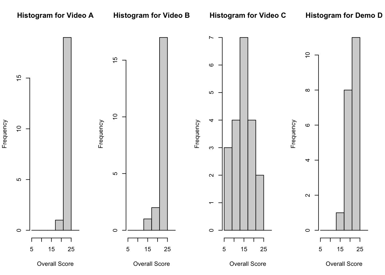
We next investigate the shapes of the group to determine the correct hypotheses.

par(mfrow=c(1,4)) 
hist(Awareness$TotalAGen, xlab='Overall Score', main='Histogram for Video A', breaks=seq(from=5,to=30, by=4)) 
hist(Awareness$TotalBdoc, xlab='Overall Score', main='Histogram for Video B', breaks=seq(from=5,to=30, by=4))
hist(Awareness$TotalCOld, xlab='Overall Score', main='Histogram for Video C', breaks=seq(from=5,to=30, by=4))
hist(Awareness$TotalDDEMO, xlab='Overall Score', main='Histogram for Demo D', breaks=seq(from=5,to=30, by=4))

The histograms show reasonably similar distribution shape, with there being a clear right skew for Video A, Video B and Demo D. We will therefore compare medians in the hypotheses for the Friedman test.

AwarenessMatrix<-matrix(c(Awareness$TotalAGen, Awareness$TotalBdoc, Awareness$TotalCOld,
        Awareness$TotalDDEMO), nrow=20,ncol=4, dimnames = list(1 : 20, c("A", "B", "C", "D")))

AwarenessMatrix

    A  B  C  D
1  25 23 13 22
2  23 23 20 22
3  20 17 14 23
4  24 24 23 25
5  25 22 18 23
6  24 22 23 25
7  25 22  9 21
8  24 23  6 21
9  25 21 11 23
10 24 23  5 25
11 24 23 15 21
12 22 24 14 19
13 24 23 14 19
14 25 25 17 18
15 24 22 14 17
16 25 23 13 20
17 25 22 16 21
18 25 21 11 22
19 25 23 19 25
20 24 23 18 25

friedman.test(AwarenessMatrix)


    Friedman rank sum test

data:  AwarenessMatrix
Friedman chi-squared = 41.372, df = 3, p-value = 5.452e-09

Clearly we have a significant result, therefore we proceed with post hoc testing.
Now a new data set is required, i.e. in a different format. We first export the matrix, create a new column containing the Awareness variable with a labelling column

write.csv(AwarenessMatrix, "Awareness.csv")

Make the changes and re-import the new dataset.

AwarenessPostHoc<-read.csv(file.choose())

We now perform the post hoc testing.

install.packages("PMCMRplus")

library(PMCMRplus)
kwAllPairsNemenyiTest(AwarenessPostHoc$Awareness~AwarenessPostHoc$Group)


    Pairwise comparisons using Tukey-Kramer-Nemenyi all-pairs test with Tukey-Dist approximation

data: AwarenessPostHoc$Awareness by AwarenessPostHoc$Group

  1      2      3     
2 0.0562 -      -     
3 3e-10  0.0003 -     
4 0.0226 0.9880 0.0011


P value adjustment method: single-step

alternative hypothesis: two.sided

This shows significant differences between Video C and Videos A and B and between Demo D and Video C.
We therefore report medians:

median(Awareness$TotalAGen)

[1] 24

median(Awareness$TotalBdoc)

[1] 23

median(Awareness$TotalCOld)

[1] 14

median(Awareness$TotalDDEMO)

[1] 22